Production Process validation: Cp, Cpk, standard deviation… statistical methods
When production quantities are large enough, it can be useful for manufacturers to validate production process, rather than performing unit tests on each device. The Production Process validation uses mathematical tools that need to be understood to use them correctly.
Note: the topic is covered in the ISO/TC 69/SC 4 series of standards.
Defining requirements on production

Before validating the manufacturing it is necessary to define requirements on the devices manufactured: these requirements are quantitative, they relate to critical physical characteristics of the product (example: a length, a diameter, a rate…)
We set:
- A nominal value (the expected value): X
- The high tolerance: USL (Upper Specification Limit)
- The low tolerance: LSL (Lower Specification Limit)
Thus, parts outside the tolerance range will be non-conform (NC).
Normal distribution of measured values
For many devices being manufactured, a measurable characteristic will vary according to a normal distribution: the distribution of measurements (the number of parts for each value range) follows a Gaussian curve :

In this example the 50 measurements are used to plot the histogram of the distribution of values, the green background covers the conforming values, the NC measurements are in the red area. Most of the points are close to the mean value.
The further the NC zone (red) is from the curve, the more likely the product is to conform
The production validation will demonstrate that:
- the curve is sufficiently narrow, so as not to exceed the tolerance zone, then the production is capable.
- the curve is sufficiently centered around the nominal value, so as not to go out of the conformity zone, then the production is repeatable.
The centering and width of the curve depend on the adjustments of the production tool and its possible drift.
Mean value and standard deviation of measured values
For a batch of n parts produced and the associated x measurements, we calculate:
- the mean value µ: Σ (measurements) / n
- the standard deviation σ : √ ( Σ( ( x – µ)² ) / n )
The mean value is easy to understand (a value “in the middle” of all measurements), the standard deviation is less intuitive: it represents how much the measurements “go all over the place”.

Probability of Conformity
It is now that the mathematical tool comes in handy: once the mean value and standard deviation have been identified it is possible to know the probability of a point being in a given value range.
The probability P of having a value in an interval around the mean value is a function of the number of standard deviations that make up that interval :
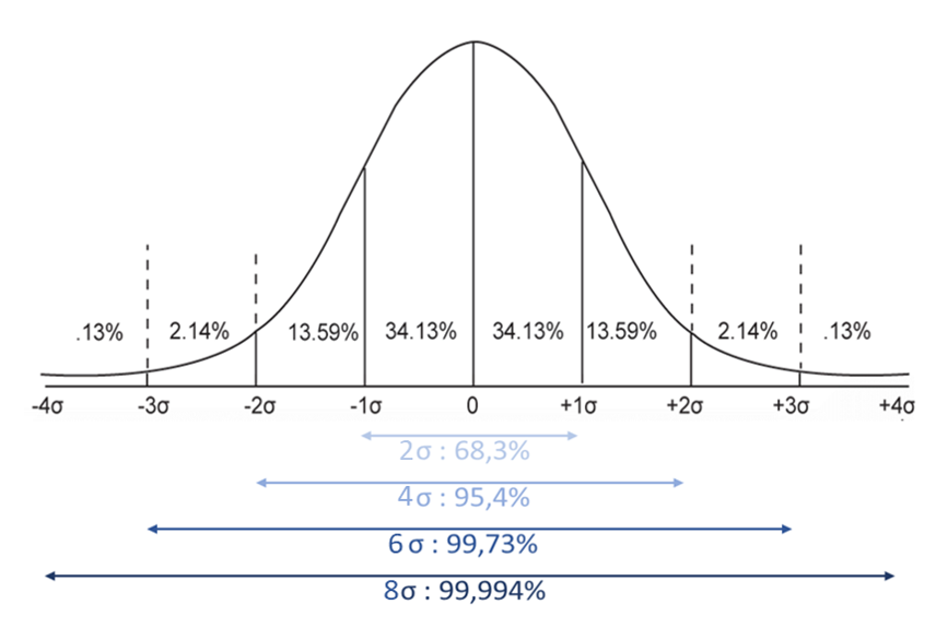
The probability that the value is outside the range (that the product is non-conform) is derived:
- x outside [-σ/2; σ/2]: 62%
- x [-σ; σ]: 32%
- x [-2σ; +2σ]: 5%
- x [-3σ; +3σ]: 0.27%
- x [-4σ; +4σ]: 0.006%
- x [-6σ; +6σ]: 0.0000002%
The goal is to have tolerances (USL and LSL) far from the mean value, typically 4σ each: with a 99.994% probability of conformity and a 66ppm (parts per million) non-conformity rate.
Capability indices Cp, Cpk, Cpm
Calculations
Indices are required to analyze production results:
- Process capability index: Cp = (USL – LSL) / 6σ
The coefficient Cp indicate “how close the tolerance range is to 6σ”: the greater Cp is, the more capable your sub-process is of producing conforming results.
With Cp = 1 the conformity range covers 6σ, the probability of being non-conform is 0.27%
With Cp = 1.33 the conformity range covers 8σ, the probability of being non-conform is 0.007%
- Minimum process capability index Cpk = min( (USL – µ)/3σ; (µ – LSL)/3σ)
The Cpk coefficient takes into account a possible dispersion of results, which despite a high Cp would make the sub-process unrepeatable.
- Machine capability: Cpm = Cp / √( 1 + 9.(Cp – Cpk)²)
The Cpm coefficient (very useful as it is very reactive) takes into account the dispersion of the results, it is commonly used to monitor the adjustment of a machine.

Useful Thresholds
The thresholds, for ruling whether the coefficients Cp, Cpk and Cpm are satisfactory, depend on the expected confidence :
Common thresholds and associated confidence probabilities are given below, a threshold of 1.33 is very often used, 1.66 indicate excellent productions (needed for large quantities of parts).
| Threshold | Sigmas (z-score) | Confidence | NC |
|---|---|---|---|
| 0.67 | 2.01 | 95.56% | 44’431 ppm |
| 1 | 3 | 99.73% | 2’700 ppm |
| 1.33 | 3.99 | 99.9934% | 66 ppm |
| 1.66 | 4.98 | 99.999936% | 1 ppm |
| 2 | 6 | 99.9999998% | 0 ppm |
The “z-score” is noted: z = 3.S
Number of samples used and induced error
We can calculate the error as a function of σ, the number of samples n and z :
e = z.σ/√n
The error will narrow the range of conformity, in effect: around the LSL values +/- 1 and USL +/- 1 values you cannot be sure that the measurement is conform.
You now have three areas: conform, Non Conformity and Unknown:

How do you use all this?
For each validation test (there is often one test per influence factor and production cycle) :
- Do a few dozen samples (typically more than 20)
- Calculate the capability indices Cpk, Cm and the error
- Continue until you have stable indices and tolerable error
You will consider the number of devices produced to set a threshold for capability indices. A high threshold – above 1.3 – will be necessary for large production runs where even low probabilities of non-conformity are critical.
The number of samples required ranges from a few dozen to several hundred depending on the standard deviation and your production volumes.
Hereafter: the evolution of the estimation of the indices and the error as a function of the number of samples, for a low standard deviation (less than 1/5 of the tolerance), we can see that the values are correctly estimated after about 40 samples:

Spreadsheet
Link to the calculation spreadsheet used to illustrate this article.